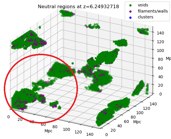
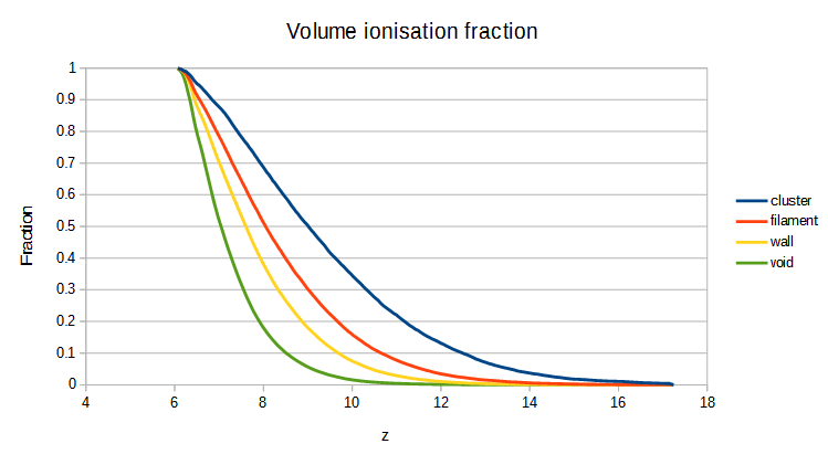
We identified the cosmic web signature (cluster, filament, wall, void) of points at z=6 and used it to study the neutral/ionised regions between 6<z<17.
Notice how the regions disappear quickly after they split off from the percolating cluster. This explains the Betti-2 persistence diagram.
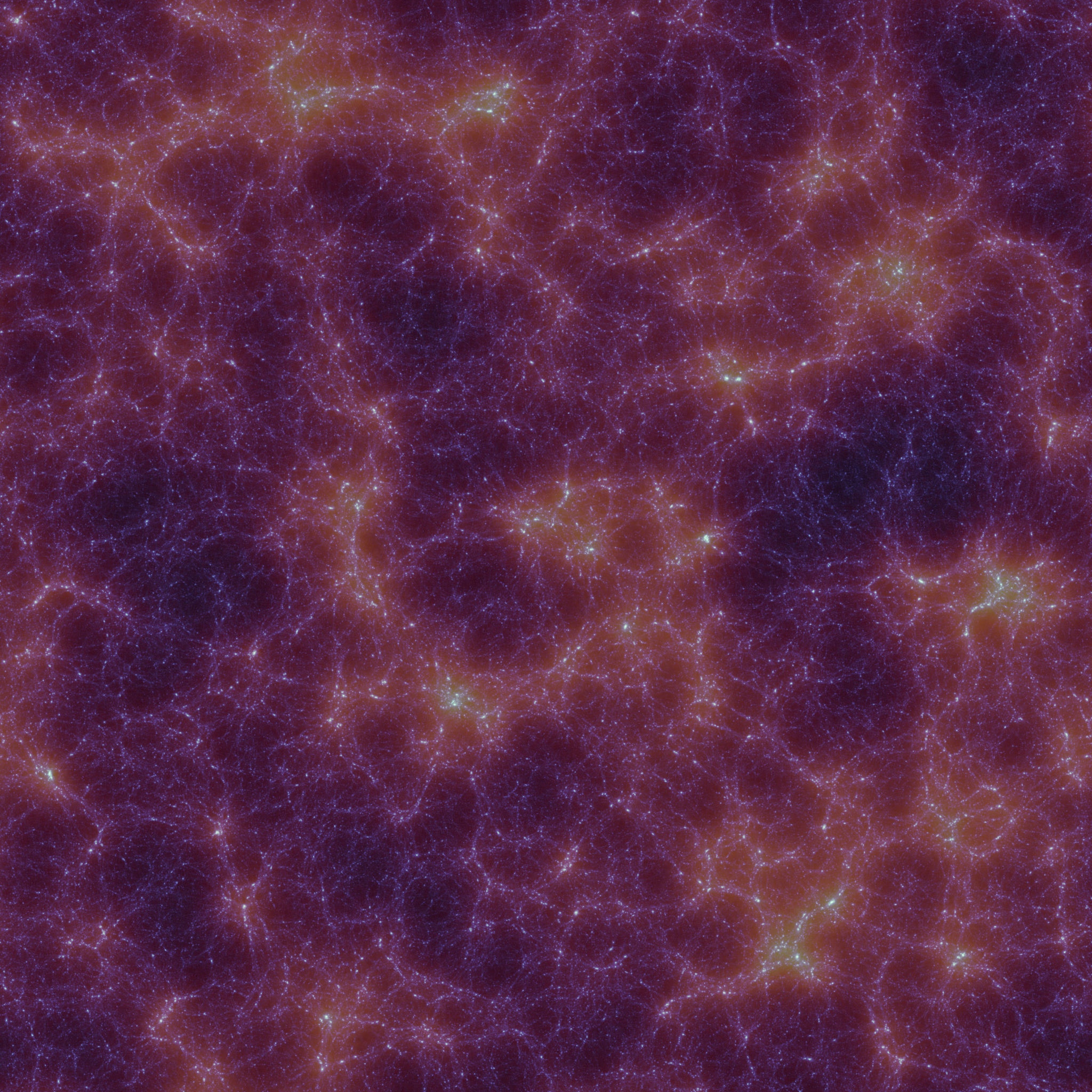
As expected, the last neutral regions largely trace the underdense regions of the cosmos, shown here as green voids. However, inside these neutral regions there do exist some clusters, filaments, and walls that are obscured from the current viewpoint. To make these visible, we adjust the draw order so that clusters are on top of filaments/walls, which are drawn on top of voids.
Here is another view that shows the locations of the clusters (regardless of their ionisation state).
Here is a snapshot from just before a number of regions split apart. Notice how two large neutral regions containing a fair number of filaments and walls (purple, most are in the interior) are connected by a neutral tunnel that passes through cosmic voids. So the neutral tunnels are not necessarily the cosmic filaments.
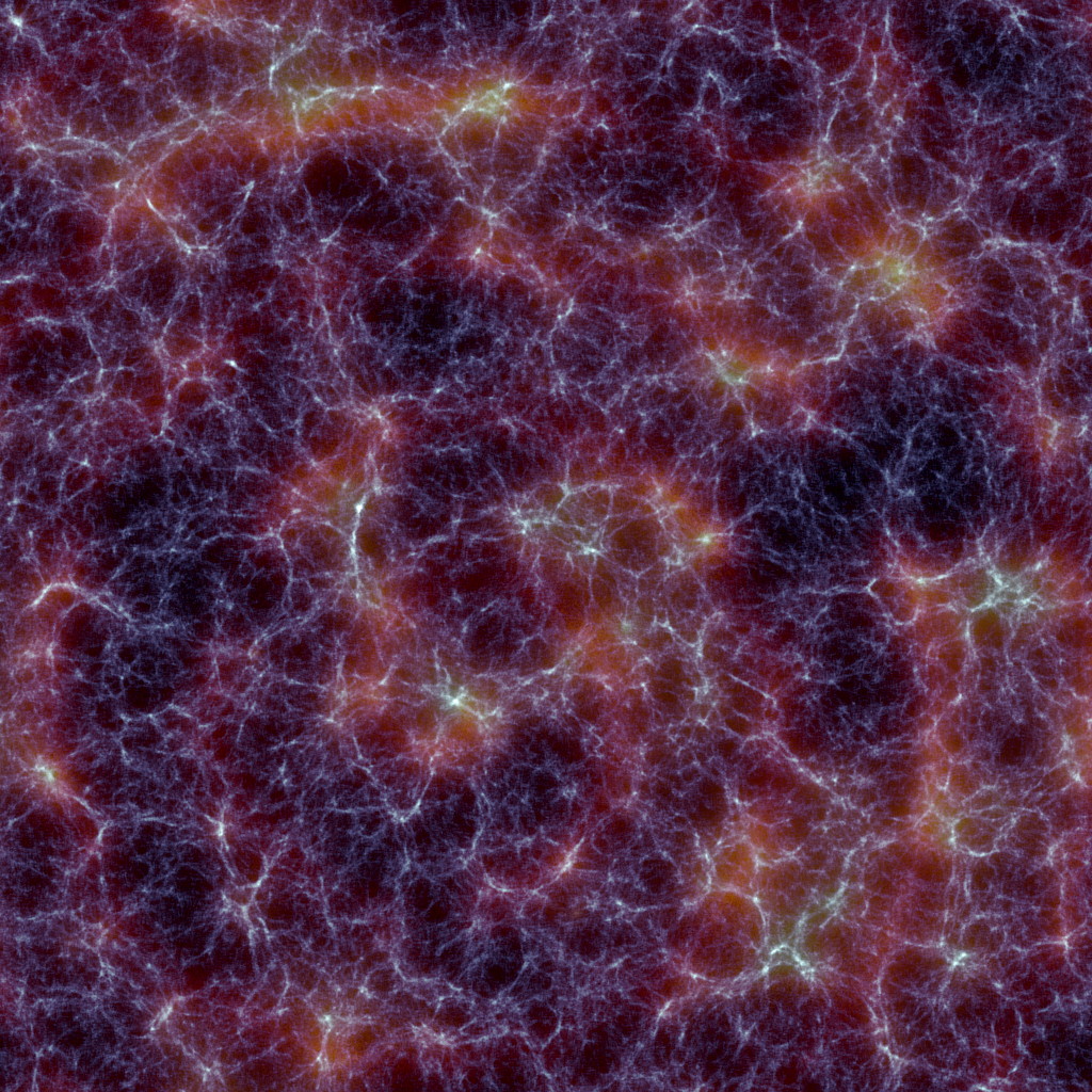
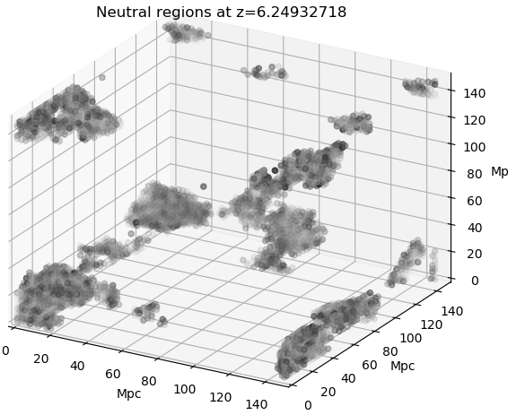
Below, the same situation but coloured according to density.
We can also look at the growth of the ionised regions.
Tip: in many browsers you can change the playback speed by right-clicking on the video.
In deriving the Lorentz invariance of the measure
$$\int\frac{\mathrm{d}^3p}{(2\pi)^3}\frac{1}{2E_\mathbf{p}},$$
the following identity is used
$$\delta\left(x^2-x_0^2\right)=\frac{1}{2|x|}\left[\delta(x-x_0)+\delta(x+x_0)\right].$$
This is proved as follows. First note that for any integrable function $f(x)$, it holds that
$$\int_{-a}^af(x)\mathrm{d}x = \int_0^a\left[f(x)+f(-x)\right]\mathrm{d}x.$$
Now, consider the change of variables $x\to x^2$ with $\mathrm{d}(x^2)=2x \mathrm{d}x$. We find that
$$\int_\infty^\infty f(x)\mathrm{d}x = \int_0^\infty \left[f\left((x^2)^{1/2}\right)+f\left(-(x^2)^{1/2}\right)\right]\frac{\mathrm{d}(x^2)}{2(x^2)^{1/2}}\\
= \int_0^\infty\left[f(| x|)+f(-| x|)\right]\frac{\mathrm{d}(x^2)}{2| x|}.$$
To prove the desired identity we now compute
$$\int_{-\infty}^\infty f(x)\delta\left(x^2-x_0^2\right)\mathrm{d}x = \int_0^\infty \left[f(| x|)+f(-| x|)\right]\delta\left(x^2-x_0^2\right)\frac{\mathrm{d}(x^2)}{2| x|}\\
= \frac{f(| x_0|) + f(-| x_0|)}{2| x_0|}.$$
We also find that
$$\int_{-\infty}^\infty f(x)\frac{\delta\left(x-x_0\right)+\delta\left(x+x_0\right)}{2| x_0|}\mathrm{d}x = \frac{f(| x_0|) + f(-| x_0|)}{2| x_0|}.$$
Because this holds for any $f$, the desired identity follows.
Given a scalar field theory described by the Lagrangian
$$\mathcal{L}=\frac{1}{2}\eta^{\mu\nu}\partial_\nu\phi\partial_\mu\phi – \frac{1}{2}m^2\phi^2,$$
we can consider the effect of an infinitesimal transformation
$$x^\mu \to x^\mu – \epsilon^\mu.$$
A quick computation shows that the change in the Lagrangian is
$$\delta\mathcal{L} = -\epsilon^\rho\partial_\rho\mathcal{L},$$
which is a total derivative. Hence, Noether’s theorem tells us that there are conserved currents for the four choices of $\epsilon_\rho$, given by
$$T^{\rho\mu} := \left(j^\rho\right)^\mu = \frac{\partial\mathcal{L}}{\partial\left(\partial_\mu\phi\right)}\partial_\rho\phi – \delta^{\mu\rho}\mathcal{L}.$$
There are then four conserved charges:
$$Q^0 = \int\mathrm{d}^3x\; T^{00} = \int\mathrm{d}^3x\left[\frac{1}{2}\dot{\phi}^2+\frac{1}{2}\left(\nabla\phi\right)^2+\frac{1}{2}m^2\phi^2\right]$$
and
$$Q^i = \int\mathrm{d}^3x\; T^{i0} = -\int\mathrm{d}^3x\;\dot{\phi}\partial^i\phi.$$
The first conserved charge is easily interpreted as the total energy: $E=Q^0$. The other three charges correspond to the total momentum in the field: $P^i=Q^i$. But does this make sense? What does the quantity $\dot{\phi}\partial^i\phi$ signify?
Well, using the symmetry of the Lagrangian under Lorentz boosts, it is possible to derive another conserved charge:
$$Q^{0i} = \int\mathrm{d}^3x\left(x^0T^{0i}-x^iT^{00}\right).$$
Since this is conserved, we find that
$$0 = \frac{\mathrm{d}Q^{0i}}{\mathrm{d}t} = \int\mathrm{d}^3x\;T^{0i}+t \int\mathrm{d}^3x\frac{\partial T^{0i}}{\partial t} – \int\mathrm{d}^3x\;x^iT^{00}\\
= P^i + t\frac{\mathrm{d}P^i}{\mathrm{d}t} – \frac{\mathrm{d}}{\mathrm{d}t} \int\mathrm{d}^3x\;x^i T^{00}.$$
Since $P^i$ is conserved, this reduces to
$$P^i = \frac{\mathrm{d}}{\mathrm{d}t}\int\mathrm{d}^3x\;x^iT^{00}.$$
This makes a lot more sense. Since $T^{00}$ is the energy density (and $E=m$), we immediately recognise the familiar rule from classical mechanics:
$$p = \frac{\mathrm{d}}{\mathrm{d}t}(mx).$$
This also suggests an interpretation for $\dot{\phi}\partial^i\phi$. Finding the expression for $T^{00}$ and taking the time derivative, we find
$$\frac{\partial}{\partial t}T^{00} = \frac{\partial}{\partial t}\left(\frac{1}{2}\dot{\phi}^2+\frac{1}{2}\left(\nabla\phi\right)^2+\frac{1}{2}m^2\phi^2\right)\\
= \dot{\phi}\ddot{\phi}+\nabla\phi(\nabla\dot{\phi})+m^2\phi\dot{\phi}.$$
We now use the equation of motion
$$\partial_\mu\partial^\mu\phi + m^2\phi = 0 \Longrightarrow \ddot{\phi} + m^2\phi = \nabla^2\phi,$$
to write this as
$$\frac{\partial}{\partial t}T^{00} = \left(\dot{\phi}\nabla^2\phi + \nabla\phi(\nabla\dot{\phi})\right) = \nabla\left(\dot{\phi}\nabla\phi\right).$$
This is a continuity equation of the form
$$\frac{\partial\rho}{\partial t} + \mathbf{\nabla}\cdot\mathbf{j} = 0,$$
where $\rho=T^{00}$ is the energy density and $\mathbf{j} = -\dot{\phi}\mathbf{\nabla}\phi$ is the energy density flux. In other words $j^i=-\dot{\phi}\partial^i\phi$ is the flow of energy in the $x^i$-direction.
Let us see how this relates to our earlier definition of $P^i$. We have
$$\frac{\mathrm{d}}{\mathrm{d}t}\left(x^iT^{00}\right) = x^i\nabla\left(\dot{\phi}\nabla\phi\right).$$
Integrating this over space, we find
$$P^i = \int\mathrm{d}^3x\;x^i\nabla\left(\dot{\phi}\nabla\phi\right).$$
Using the divergence theorem, we have in general for scalar functions $u,v,w$ that
$$\int\mathrm{d}^3x\;u\nabla\cdot\left(v\nabla w\right) = -\int\mathrm{d}^3x\;\nabla u\cdot\left(v\nabla w\right) + \text{boundary term}.$$
Hence, in our case, we find
$$P^i = -\int\mathrm{d}^3x\;\dot{\phi}\partial^i\phi,$$
which is what we had originally. So indeed, the total momentum of the scalar field in the $x^i$-direction is simply the energy flux in the $x^i$-direction integrated over all space.
In Peskin and Schroeder’s Introduction to Quantum Field Theory, the quantisation of the free scalar field is done by analogy with the classical one-dimensional harmonic oscillator, which is described by the Hamiltonian
$$H=\frac{1}{2}p^2 + \frac{1}{2}\omega^2x^2,$$
where $p$ is the momentum and $x$ the displacement of the oscillator. The standard ansatz is to expand the momentum and position operators in terms of ladder operators:
$$x = \frac{1}{\sqrt{2\omega}} \left(a+a^\dagger\right), \;\,\;\,\;\, p = -i\sqrt{\frac{\omega}{2}} \left(a-a^\dagger\right),$$
which can easily be inverted to give
$$a = \sqrt{\frac{\omega}{2}}q + \frac{i}{\sqrt{2\omega}}p, \;\,\;\,\;\, a^\dagger = \sqrt{\frac{\omega}{2}}q\; – \frac{i}{\sqrt{2\omega}}p.$$
With these relations in hand, it is not difficult to prove that the commutation relations
$$[x,x]=[p,p]=0,\;\,\;\,\;\, [x,p]=i$$
are equivalent to
$$[a,a]=[a^\dagger,a^\dagger]=0,\;\,\;\,\;\, [a,a^\dagger]=1.$$
For the scalar field $\phi(\mathbf{x})$ and its momentum conjugate $\pi(\mathbf{x})$, we can do something similar by expanding their Fourier transforms in terms of ladder operators:
$$\phi(\mathbf{x}) = \int\frac{\mathrm{d}^3p}{(2\pi)^3}\frac{1}{\sqrt{2\omega}}\left[a_\mathbf{p}e^{i\mathbf{p}\cdot\mathbf{x}}+a_\mathbf{p}^\dagger e^{-i\mathbf{p}\cdot\mathbf{x}}\right],\\
\pi(\mathbf{x}) = -i\int\frac{\mathrm{d}^3p}{(2\pi)^3}\sqrt{\frac{\omega}{2}}\left[a_\mathbf{p}e^{i\mathbf{p}\cdot\mathbf{x}}-a_\mathbf{p}^\dagger e^{-i\mathbf{p}\cdot\mathbf{x}}\right].$$
Given the commutation relations
$$[a_\mathbf{p},a_\mathbf{q}]=[a_\mathbf{p}^\dagger,a_\mathbf{q}^\dagger]=0,\\
[a_\mathbf{p},a_\mathbf{q}^\dagger]=(2\pi)^3\delta^{(3)}(\mathbf{p}-\mathbf{q}),$$
it is now straightforward to prove the relations
$$[\phi(\mathbf{x}),\phi(\mathbf{y})]=[\pi(\mathbf{x}),\pi(\mathbf{y})]=0,\\
[\phi(\mathbf{x}),\pi(\mathbf{y})]=i\delta^{(3)}(\mathbf{x}-\mathbf{y}).$$
However, the reverse implication is not immediately obvious and is not proved in the book, even though it seems more natural to assume the canonical commutation relation and then derive the commutators for the ladder operators. To prove the reverse direction, first assume that the commutation relations for $\phi(\mathbf{x})$ and $\pi(\mathbf{x})$ hold. We write
$$0 = [\phi(\mathbf{x}),\phi(\mathbf{y})] = \int\frac{\mathrm{d}^3p}{(2\pi)^3}\frac{\mathrm{d}^3q}{(2\pi)^3}\frac{1}{2\sqrt{\omega_\mathbf{p}\omega_\mathbf{q}}}\left[[a_\mathbf{p},a_\mathbf{q}]e^{i(\mathbf{p}\cdot\mathbf{x}+\mathbf{q}\cdot\mathbf{y})}+[a^\dagger_\mathbf{p},a_\mathbf{q}]e^{i(-\mathbf{p}\cdot\mathbf{x}+\mathbf{q}\cdot\mathbf{y})}\right.\\
\left.+[a_\mathbf{p},a^\dagger_\mathbf{q}]e^{i(\mathbf{p}\cdot\mathbf{x}-\mathbf{q}\cdot\mathbf{y})}+[a^\dagger_\mathbf{p},a^\dagger_\mathbf{q}]e^{i(-\mathbf{p}\cdot\mathbf{x}-\mathbf{q}\cdot\mathbf{y})}\right],\\
0 = [\pi(\mathbf{x}),\phi(\mathbf{y})] = -\int\frac{\mathrm{d}^3p}{(2\pi)^3}\frac{\mathrm{d}^3q}{(2\pi)^3}\frac{\sqrt{\omega_\mathbf{p}\omega_\mathbf{q}}}{2}\left[[a_\mathbf{p},a_\mathbf{q}]e^{i(\mathbf{p}\cdot\mathbf{x}+\mathbf{q}\cdot\mathbf{y})}-[a^\dagger_\mathbf{p},a_\mathbf{q}]e^{i(-\mathbf{p}\cdot\mathbf{x}+\mathbf{q}\cdot\mathbf{y})}\right.\\
\left.-[a_\mathbf{p},a^\dagger_\mathbf{q}]e^{i(\mathbf{p}\cdot\mathbf{x}-\mathbf{q}\cdot\mathbf{y})}+[a^\dagger_\mathbf{p},a^\dagger_\mathbf{q}]e^{i(-\mathbf{p}\cdot\mathbf{x}-\mathbf{q}\cdot\mathbf{y})}\right].$$
Because we integrate over the entire domain and because $\omega_\mathbf{p}=\omega_{-\mathbf{p}}$, we are allowed to substitute $-\mathbf{p}$ for $\mathbf{p}$ (and similarly for $\mathbf{q}$) in any of the four terms within the brackets. This gives us the following relation
$$0 = \int\frac{\mathrm{d}^3p}{(2\pi)^3}\frac{\mathrm{d}^3q}{(2\pi)^3} \left[f_1(\mathbf{p},\mathbf{q})e^{i(\mathbf{p}\cdot\mathbf{x}+\mathbf{q}\cdot\mathbf{y})}+f_2(\mathbf{p},\mathbf{q})e^{-i(\mathbf{p}\cdot\mathbf{x}-\mathbf{q}\cdot\mathbf{y})}+f_3(\mathbf{p},\mathbf{q})e^{-i(\mathbf{p}\cdot\mathbf{x}+\mathbf{q}\cdot\mathbf{y})}\right]\\
= \int\frac{\mathrm{d}^3p}{(2\pi)^3}\frac{\mathrm{d}^3q}{(2\pi)^3} \left[g_1(\mathbf{p},\mathbf{q})e^{i(\mathbf{p}\cdot\mathbf{x}+\mathbf{q}\cdot\mathbf{y})}+g_2(\mathbf{p},\mathbf{q})e^{-i(\mathbf{p}\cdot\mathbf{x}-\mathbf{q}\cdot\mathbf{y})}+g_3(\mathbf{p},\mathbf{q})e^{-i(\mathbf{p}\cdot\mathbf{x}+\mathbf{q}\cdot\mathbf{y})}\right],$$
where I have introduced the functions
$$f_1(\mathbf{p},\mathbf{q})=\frac{[a_\mathbf{p},a_\mathbf{q}]}{\sqrt{\omega_\mathbf{p}\omega_\mathbf{q}}}, \;\,\;\,\;\, f_2(\mathbf{p},\mathbf{q})=\frac{[a^\dagger_\mathbf{p},a_\mathbf{q}] + [a_{-\mathbf{p}},a^\dagger_{-\mathbf{q}}]}{\sqrt{\omega_\mathbf{p}\omega_\mathbf{q}}}, \;\,\;\,\;\, f_3(\mathbf{p},\mathbf{q})=\frac{[a^\dagger_\mathbf{p},a^\dagger_\mathbf{q}]}{\sqrt{\omega_\mathbf{p}\omega_\mathbf{q}}},\\
g_1(\mathbf{p},\mathbf{q})=\omega_\mathbf{p}\omega_\mathbf{q}\;f_1(\mathbf{p},\mathbf{q}), \;\,\;\,\;\, g_2(\mathbf{p},\mathbf{q})=-\omega_\mathbf{p}\omega_\mathbf{q}\;f_2(\mathbf{p},\mathbf{q}), \;\,\;\,\;\, g_3(\mathbf{p},\mathbf{q})=\omega_\mathbf{p}\omega_\mathbf{q}\;f_3(\mathbf{p},\mathbf{q}).$$
The takeaway is that because the exponentials $\exp(\pm i\mathbf{p}\cdot\mathbf{x}\pm i\mathbf{q}\cdot\mathbf{y})$ are linearly independent, we must have that $f_i(\mathbf{p},\mathbf{q})=g_i(\mathbf{p},\mathbf{q})=0$. Hence, we find in particular that
$$[a_\mathbf{p},a_\mathbf{q}]=[a_\mathbf{p}^\dagger,a_\mathbf{q}^\dagger]=0.$$
Deriving the final commutator takes some more work. We start with the third relation between $\phi(\mathbf{x})$ and $\pi(\mathbf{y})$:
$$i\delta^{(3)}(\mathbf{x}-\mathbf{y})=[\phi(\mathbf{x}),\pi(\mathbf{y})] = \frac{-i}{2}\int\frac{\mathrm{d}^3p}{(2\pi)^3}\frac{\mathrm{d}^3q}{(2\pi)^3}\left[[a_\mathbf{p},a_\mathbf{q}]e^{i(\mathbf{p}\cdot\mathbf{x}+\mathbf{q}\cdot\mathbf{y})}-[a^\dagger_\mathbf{p},a_\mathbf{q}]e^{i(-\mathbf{p}\cdot\mathbf{x}+\mathbf{q}\cdot\mathbf{y})}\right.\\
\left.+[a_\mathbf{p},a^\dagger_\mathbf{q}]e^{i(\mathbf{p}\cdot\mathbf{x}-\mathbf{q}\cdot\mathbf{y})}-[a^\dagger_\mathbf{p},a^\dagger_\mathbf{q}]e^{i(-\mathbf{p}\cdot\mathbf{x}-\mathbf{q}\cdot\mathbf{y})}\right]\\
= \frac{-i}{2}\int\frac{\mathrm{d}^3p}{(2\pi)^3}\frac{\mathrm{d}^3q}{(2\pi)^3}\left[-[a^\dagger_\mathbf{p},a_\mathbf{q}]e^{i(-\mathbf{p}\cdot\mathbf{x}+\mathbf{q}\cdot\mathbf{y})}+[a_\mathbf{p},a^\dagger_\mathbf{q}]e^{i(\mathbf{p}\cdot\mathbf{x}-\mathbf{q}\cdot\mathbf{y})}\right].$$
Multiplying the left hand side by $\int\mathrm{d}^3x\;\mathrm{d}^3y\; e^{-i(\mathbf{p’}\cdot\mathbf{x}+\mathbf{q’}\cdot\mathbf{y})}$ gives
$$\int\mathrm{d}^3x\;\mathrm{d}^3y\; e^{-i(\mathbf{p’}\cdot\mathbf{x}+\mathbf{q’}\cdot\mathbf{y})}i\delta^{(3)}(\mathbf{x}-\mathbf{y})=\int\mathrm{d}^3y\; e^{-i(\mathbf{p’}+\mathbf{q’})\cdot\mathbf{y}}i(2\pi)^3\\
=i\delta^{(3)}(\mathbf{p’}-\mathbf{q’})(2\pi)^3.$$
The right hand side becomes
$$-\frac{i}{2}\int\mathrm{d}^3x\;\mathrm{d}^3y\frac{\mathrm{d}^3p}{(2\pi)^3}\frac{\mathrm{d}^3q}{(2\pi)^3}\left[-[a^\dagger_\mathbf{p},a_\mathbf{q}]e^{i(-(\mathbf{p}+\mathbf{p’})\cdot\mathbf{x}+(\mathbf{q}-\mathbf{q’})\cdot\mathbf{y})}+[a_\mathbf{p},a^\dagger_\mathbf{q}]e^{i((\mathbf{p}-\mathbf{p’})\cdot\mathbf{x}-(\mathbf{q}+\mathbf{q’})\cdot\mathbf{y})}\right]\\
=-\frac{i}{2}\left[-[a^\dagger_{-\mathbf{p’}},a_\mathbf{q’}]+[a_\mathbf{p’},a^\dagger_{-\mathbf{q’}}]\right]\\
=i[a^\dagger_{-\mathbf{p’}},a_\mathbf{q’}],$$
where we used $f_2(\mathbf{p},\mathbf{q})=g_2(\mathbf{p},\mathbf{q})=0$ in the final step. It follows that
$$\delta^{(3)}(\mathbf{p}-\mathbf{q})(2\pi)^3 = [a^\dagger_\mathbf{p},a_\mathbf{q}],$$
if we simply substitute $\mathbf{p}$ for $-\mathbf{p’}$ and $\mathbf{q}$ for $\mathbf{q’}$. This is what we wanted to show.